Deep Research Agent – Autonomous AI Research Assistant

ai agent

Abstract As Large Language Models (LLMs) evolve from simple text generators to reasoning engines, the focus of AI development has shifted toward agentic workflows—systems capable of autonomous planning, tool use, and self-correction. To explore the efficacy of modern orchestration frameworks, I engineered the Deep Research Agent: a fully autonomous system designed to perform iterative, multi-step research tasks. This project demonstrates a production-ready implementation of a cyclic graph architecture (LangGraph) utilizing the Groq API for high-throughput inference. The resulting system achieves professional-grade research synthesis with a marginal operating cost of $0.005 per query, proving that high-performance autonomous agents can be built cost-effectively using open-weight models. 1. System Overview: The Deep Research Agent The Deep Research Agent is not merely a wrapper for an LLM; it is a stateful application that mimics the workflow of a human analyst. Unlike zero-shot querying, this system employs an iterative “thought-loop” to refine information quality before generating a final response. Core Capabilities: 2. Technical Stack & Design Choices The architecture was chosen to maximize architectural flexibility while minimizing inference latency and operational costs. 3. Architectural Analysis: Cyclic Graph vs. Linear Chains A key engineering decision in this project was the implementation of a Cyclic Graph architecture over a traditional Linear Chain. 4. Engineering Implementation & Challenges The development process highlighted several critical aspects of building production-grade agents. A. State Management Implementation Effective state management is the backbone of any agentic system. I implemented a TypedDict structure with reducer operators to maintain context across iterations. This ensures that research findings are accumulated rather than overwritten during loops. Python B. Resilience and Error Handling To ensure robustness suitable for automated tasks, I implemented exponential backoff strategies for all external API calls. This prevents cascade failures during momentary latency spikes from search or LLM providers. Python C. Resource Optimization (Cost Analysis) A primary objective was to demonstrate the economic feasibility of running autonomous agents at scale. By optimizing the system prompt and pruning search results (limiting context window usage), the system achieves a 95% cost reduction compared to proprietary model APIs (e.g., GPT-4). Metric Standard API approach Deep Research Agent (Optimized) Cost Per Query ~$0.10 **~$0.005** Latency Variable < 3s (Inference) Architecture Black Box Open / Customizable 5. Conclusion & Future Scope This project validates that professional-grade AI agents do not require prohibitive budgets or closed ecosystems. By leveraging LangGraph for sophisticated orchestration and Groq for high-speed inference, I have engineered a system that is both autonomous and economically scalable. Future Research Directions: Repository: github.com/kazisalon/Deep-Research-Agent

Understanding F1 Score in Machine Learning

f1 score machine learning

The F1 score is a crucial metric in the field of machine learning, particularly in the evaluation of classification models. It provides a balance between precision and recall, making it especially useful in scenarios where the class distribution is imbalanced. This document will delve into the definition, calculation, and significance of the F1 score, along with its applications in various domains. What is F1 Score? The F1 score is the harmonic mean of precision and recall. It is defined as follows: Where: The F1 score is then calculated using the formula: [ F1 = 2 \times \frac{\text{Precision} \times \text{Recall}}{\text{Precision} + \text{Recall}} ] Importance of F1 Score The F1 score is particularly important in the following scenarios: Applications of F1 Score The F1 score is widely used in various domains, including: Conclusion In summary, the F1 score is an essential metric in machine learning that provides a balanced measure of a model’s precision and recall. Its significance is particularly pronounced in scenarios involving imbalanced datasets and varying costs of prediction errors. Understanding and utilizing the F1 score can lead to better model evaluation and selection, ultimately enhancing the effectiveness of machine learning applications.

Recursive Induction of Decision Trees: A Building Block of Random Forest

Recursive Induction of Decision Trees

Decision trees are a fundamental building block in machine learning, particularly in the context of ensemble methods like Random Forest. A decision tree is a tree-like model of decisions and their possible consequences, including chance event outcomes, resource costs, and utility. In machine learning, decision trees are used to classify or predict outcomes based on a set of input features.   Recursive Induction: The Core Process The process of building a decision tree is known as recursive partitioning or recursive induction. It involves the following steps: Key Concepts in Decision Tree Induction Advantages of Decision Trees Limitations of Decision Trees Conclusion Recursive induction is a powerful technique for building decision trees. By understanding the principles of feature selection, splitting criteria, and stopping conditions, you can effectively construct accurate and interpretable decision trees. While decision trees can be used as standalone models, they are often combined with other techniques like bagging and boosting to create more robust and powerful ensemble models like Random Forest.

Random Forest in Machine Learning

Random Forest in Machine Learning

Random Forest is a versatile and robust machine learning algorithm that belongs to the family of ensemble learning methods. It combines multiple decision trees to create a more accurate and stable predictive model. How Random Forest Works Key Advantages of Random Forest Applications of Random Forest Limitations of Random Forest Conclusion Random Forest is a powerful and flexible machine learning algorithm that has proven its effectiveness in a wide range of applications. Its ability to handle large datasets, reduce overfitting, and provide feature importance makes it a valuable tool in the data scientist’s arsenal. By understanding its strengths and limitations, you can effectively apply Random Forest to solve complex machine learning problems.

Gradient Boosting vs. Random Forest: A Comparative Analysis

Gradient Boosting vs. Random Forest

Gradient Boosting and Random Forest are two powerful ensemble learning techniques that have become essential tools in the machine learning practitioner’s toolkit. Both methods combine multiple base models to create a more accurate and robust predictive model. However, they differ significantly in their underlying principles and performance characteristics.   Random Forest A Random Forest is an ensemble learning method that operates by constructing multiple decision trees during training and outputting the class that is the mode of the classes (classification) or mean prediction (regression) of the individual trees. Key characteristics of Random Forest include:   Gradient Boosting Gradient Boosting is a sequential ensemble method that builds models sequentially, with each new model focusing on correcting the errors of the previous models. Key characteristics of Gradient Boosting include:   Key Differences Feature Random Forest Gradient Boosting Model Building Parallel Sequential Error Correction Not explicit Explicitly corrects errors of previous models Bias-Variance Trade-off High bias, low variance Low bias, high variance Sensitivity to Outliers Less sensitive More sensitive Interpretability More interpretable Less interpretable Export to Sheets Choosing the Right Algorithm The choice between Gradient Boosting and Random Forest depends on several factors: In many cases, both algorithms can achieve high performance. It’s often beneficial to experiment with both and compare their results on a specific dataset. Conclusion Both Random Forest and Gradient Boosting are powerful ensemble methods that have proven to be effective in a wide range of machine learning tasks. By understanding their strengths and weaknesses, you can make informed decisions about when to use each technique.   Sources and related content

RNN in Machine Learning

RNN in Machine Learning

Introduction In the realm of machine learning, Recurrent Neural Networks (RNNs) have emerged as a powerful tool for modeling sequential data. Unlike traditional neural networks, which process data independently, RNNs possess a unique ability to consider the order and context of data points. This makes them ideal for tasks such as natural language processing, speech recognition, and time series analysis. Understanding RNNs At the core of RNNs is the concept of a recurrent connection. This connection allows information to persist across time steps, enabling the network to capture long-term dependencies in the data. A basic RNN unit, often referred to as a recurrent cell, consists of: The hidden state is updated at each time step based on the current input and the previous hidden state. This update mechanism allows the network to learn and remember patterns in the data.   Types of RNNs Applications of RNNs RNNs have numerous applications across various domains: Challenges and Future Directions While RNNs have achieved significant success, they still face challenges: To address these challenges, researchers are exploring various techniques: Conclusion Recurrent Neural Networks have revolutionized the field of machine learning by enabling the modeling of sequential data. With their ability to capture complex patterns and dependencies, RNNs continue to drive innovation in various applications. As research progresses and new techniques emerge, we can expect even more powerful and sophisticated RNN-based models in the future.

Genetic Algorithm in Machine Learning

Genetic Algorithm in Machine Learning

Introduction In the realm of machine learning, algorithms inspired by natural processes have proven to be remarkably effective. One such algorithm, the Genetic Algorithm (GA), draws inspiration from the principles of natural selection and genetic inheritance. This powerful optimization technique has gained significant attention for its ability to solve complex problems, particularly in areas where traditional methods fall short. Understanding Genetic Algorithms A genetic algorithm operates on a population of potential solutions, often referred to as individuals or chromosomes. Each individual is represented as a string of binary digits or a sequence of parameters. The algorithm iteratively improves this population through a process of selection, crossover, and mutation. Applications of Genetic Algorithms in Machine Learning Genetic algorithms have a wide range of applications in machine learning, including: Advantages of Genetic Algorithms Challenges and Considerations While genetic algorithms offer numerous advantages, they also present some challenges: Conclusion Genetic algorithms have emerged as a powerful tool in the machine learning toolbox. By drawing inspiration from natural processes, they provide a robust and flexible approach to solving complex optimization problems. As computational resources continue to grow and algorithmic techniques advance, genetic algorithms are poised to play an even more significant role in the future of machine learning.

Traffic Sign Classification Project with Deep Learning

Traffic Sign Classification

Introduction Traffic signs are crucial for ensuring road safety and guiding drivers. With self-driving cars and intelligent transportation systems becoming more common, automating the recognition of traffic signs is vital. This project, “Traffic Sign Classification,” leverages deep learning to identify traffic signs from images, laying the groundwork for safer roadways. Want to explore this project hands-on? You can access the complete implementation on Google Colab. Click the link below to get started: https://colab.research.google.com/drive/1bFTRr0ULw53CXL0uUGhGHIV3taU4p8cs?usp=sharing Dataset Overview The [mention dataset name, e.g., German Traffic Sign Recognition Benchmark (GTSRB)] dataset was used for this project. It contains thousands of labeled images of traffic signs in different categories. Loading the Dataset Data Preprocessing To ensure high model performance, the dataset was preprocessed with techniques like normalization, resizing, and data augmentation. Normalizing and Resizing Images Data Augmentation Model Architecture A convolutional neural network (CNN) was employed for traffic sign classification. Below is an example of the model architecture. Building the CNN Model Training the Model The model was trained over multiple epochs to minimize loss and improve accuracy. Training Code Results The model achieved a test accuracy of [insert accuracy]. Below is the confusion matrix visualizing the model’s performance. Visualizing Predictions Applications This project has real-world applications in: Conclusion The “Traffic Sign Classification” project demonstrates the power of deep learning in solving critical road safety challenges. Future improvements could include real-time detection and recognition systems to further enhance its robustness.

Sigmoid Neurons in Deep Learning

Sigmoid Neurons in Deep Learning

sigmoid neuron, deep learning, neural network, activation function, non-linearity, machine learning, backpropagation, ReLU, vanishing gradient problem